Sensing stiction
Drs. Wilfred T. Tysoe & Nicholas D. Spencer, Contributing Editors | TLT Cutting Edge October 2022
Careful, low-speed sliding experiments reveal the origins of static friction and why it is so hard to measure.

Perhaps the first thing we learn as budding tribologists is about static and dynamic friction coefficients,
μS and
μd, where the initially large force required to initiate motion reduces to a lower constant value needed to keep things going. A common explanation for this behavior is that the static contact area slowly increases when the system is at rest, making the contact hard to shear, and the dynamics are often described by so-called state-rate theories.
1 However, as recently pointed out by professor Daniel Bonn and co-worker Dr. Kasra Farain, from the University of Amsterdam, static friction and the contact area can evolve in opposite directions, and slipping can actually cause the real contact area to grow.
2
To study static friction in greater detail, they carried out careful experiments by rubbing a polytetrafluoroethylene (PTFE) sphere of 3.18 mm in diameter and approximately 1.5 μm rms roughness on smooth (<1 nm rms roughness) glass at a speed of ~4 μm/s to reveal a distinct initial static friction, which decayed over several seconds to a constant value
(see Figure 1, pink curve). The decay time increases with slower sliding
(see Figure 1, red curve), but the transient disappears completely when the experiment is repeated immediately
(see Figure 1, gray curve), and only reappears after a long wait; the interface “remembers” what happened during the previous run.
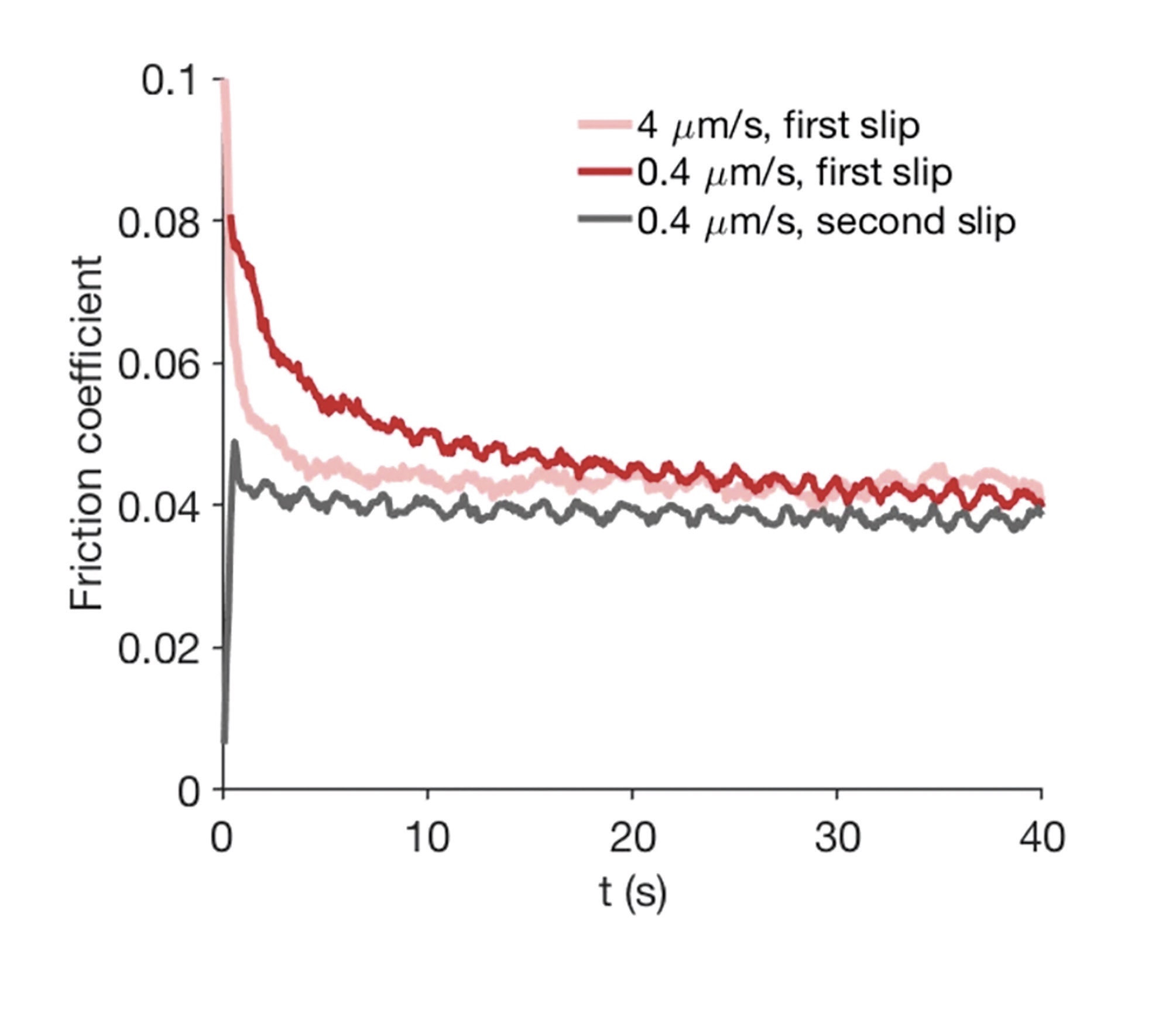 Figure 1. Transient friction at the onset of sliding for PTFE on glass. At high sliding velocities, friction starts above the steady-state value but gradually decays to a steady state, via a slow transient. The second run of the same system (gray curve) shows no transient. Published with permission from Reference 2.
To gain further insights into this behavior, experiments were performed at a very slow sliding speed (1 nm/s) for long times
(see Figure 2). Now the friction reaches its maximum value after ~1,000s and then decreases but resembles the high-velocity data
(from Figure 1) when both results are plotted as a function of distance. These results cannot be analyzed using conventional rate-state theory, and Drs. Bonn and Farain proposed that the behavior was the result of a competition between contact aging and rejuvenation; the evolution in friction force is given by
dF/dt=Rate(Aging)-Rate(Rejuvenation). They developed a phenomenological model where
Rate(Aging)=a/t, where
a is a constant. The rejuvenation rate is assumed to depend on how far the force is from the steady-state value,
Fd, and on the sliding velocity:
Rate(Rejuvenation)=αv(F-Fd ), where
α is another constant. Combining these formulae and writing the equation as a function of the sliding distance
x=vt: dF/dx = a/x - α(F-Fd) (1) shows that the friction responses should depend only on the sliding distance, as emphasized by Figure 2. The linear velocity dependence of rejuvenation is confirmed by the results shown in Figure 3, which also shows results for similar experiments on polypropylene.
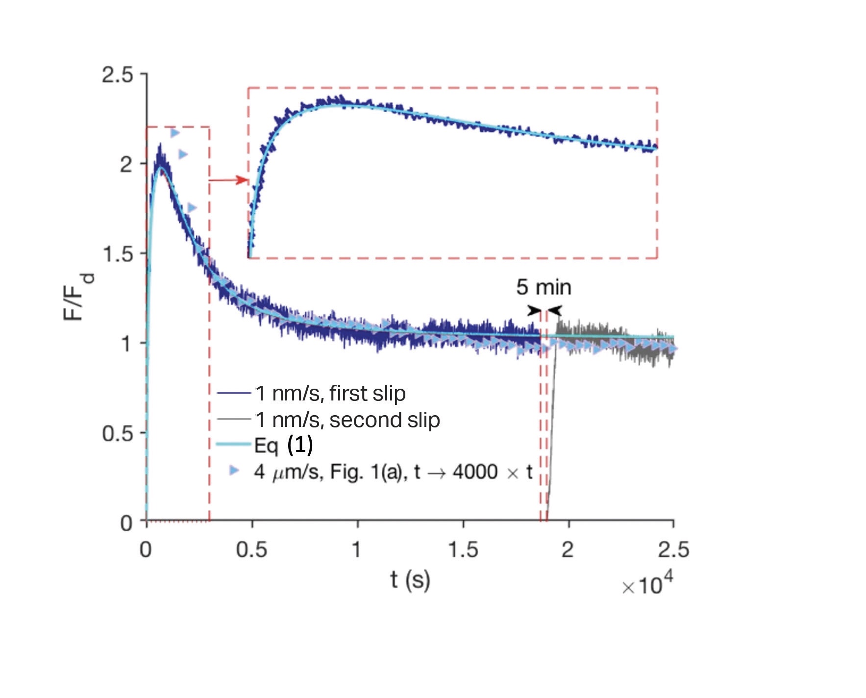 Figure 2. Slow friction dynamics for PTFE sphere on glass surface at 1 nm/s. It takes approximately 5 h for the frictional system to reach the steady-state dynamic friction. A second sliding run, started 5 min after the first run, also is shown (gray line). Cyan solid line is a fit to Equation 1. The inset shows the timeframe from 0 to 3,000s. Triangles are data from Figure 1, 4μm/s, when the time axis is extended 4,000 times. This implies that, while the transient dynamics occur over very different time scales (2-3 s versus 25,000 s), they are similar when plotted as a function of sliding distance. Published with permission from Reference 2.
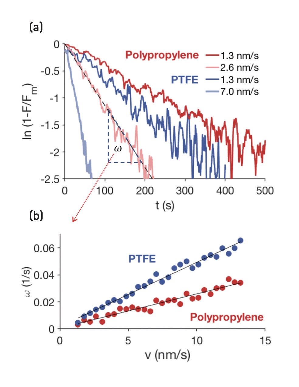
Figure 3. The increasing slow-sliding dynamics can be approximated by: ln(1-F/Fm )=ωt, with ω being proportional to v, and Fm is the maximum friction in agreement with Equation 1. Published with permission from Reference 2.
Equation 1 can be solved analytically, and the results are in good agreement with the experiment
(see Figure 2, cyan line). However,
F(t) depends on the time during which the system initially evolves but is infinite when the delay time →0. In practice, that does not occur, but it indicates that small variations in delay time can result in large differences in the subsequent friction. This is consistent with the observation that static friction coefficients are very difficult to reproduce experimentally. It also explains why it is easier to move a large piece of furniture by first jiggling it a bit.
REFERENCES
1.
Tysoe, W. T. and Spencer, N. D. (2017), “Modeling miniature earthquakes,” TLT,
73 (2), pp. 86-87. Available
here.
2.
Farain, K. and Bonn, D. (2022), “Nonmonotonic dynamics in the onset of frictional slip,”
Tribology Letters, 70, 57.
Eddy Tysoe is a distinguished professor of physical chemistry at the University of Wisconsin-Milwaukee. You can reach him at wtt@uwm.edu.
Nic Spencer is emeritus professor of surface science and technology at the ETH Zurich, Switzerland, and editor-in-chief of STLE-affiliated Tribology Letters journal. You can reach him at nspencer@ethz.ch.