Augmenting Archard
Drs. Wilfred T. Tysoe & Nicholas D. Spencer, Contributing Editors | TLT Cutting Edge August 2022
A cunning model and a touch of inspiration combine with a simple measurement to make the Archard equation even more useful.

The Archard equation
1 is stunning in its simplicity and usefulness. It relies on breathtaking approximations to describe wear rates with reasonable accuracy under a host of different conditions and for a plethora of different wear mechanisms. While it is widely used in engineering practice, it is generally not applied until the running-in period is complete and a steady state has been reached
(see Figure 1).
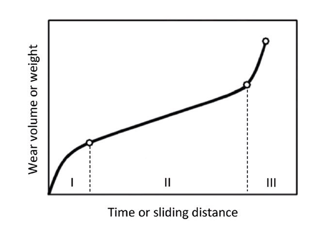
Figure 1. Typical wear curve. (I) Running-in stage. (II) Steady-state wear stage. (III) Wear-out stage. Reproduced from Ref. 3 with kind permission.
Generally this is not a significant problem, but in cases where any significant wear is unacceptable (e.g., with thin coatings), Archard can typically not be applied, since during the running-in phase, the initial surface roughness will play a crucial role, as was already pointed out half a century ago.
2
STLE member Dr. Michael Varenberg, working at John Crane Inc. in Morton Grove, Ill., has considered this problem from a new angle,
3 with the help of another handy tribological tool, the bearing-ratio (b-r) curve (or Abbott-Firestone curve
4), which, without making assumptions about the surface, describes the relationship between the height of the surface and contact area, and is readily obtained from profilometry. The running-in period can be thought of as a phase during which every point on the surface experiences contact and wear at some moment. In fact, the entire surface region characterized prior to wearing (from the highest to the lowest point,
Rt in Figure 2) is consumed during running in, as the surface is transformed into the steady-state roughness profile. This idea was already suggested,
2 but the question remains as to how long this process takes.
The method is as follows: firstly, the Archard equation is expressed in terms of the area of the worn surface, which increases from 0% to 100% as the material is removed, as illustrated in Figure 2, which also shows the corresponding b-r curve. Thus, if an imaginary truncation line is lowered through the roughness profile, the fraction that is lying within the material is designated the material ratio,
Mr, which changes from 0% to 100% as a function of height,
h. An obvious next step in the wear analysis would be to use a real b-r curve, but a novel approach introduced by Varenberg is to model the curve with a “logistic” function borrowed from population-growth studies.
5 This leads to:
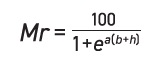
where the constants
a and
b describe the curve’s steepness and height at the midpoint. They can be obtained by calibrating against a measured b-r curve; substituting the coordinates defining the core height into this equation yields an expression for a in terms of
Rk, Mr1 and
Mr2, all of which are standard output parameters from a modern profiler.
b is the distance from the origin to the height at which the
Mr is 50%, i.e.,
Rδc(0%-50%), which is the sum of
Rk/2 and
Rpk*—also readily obtained from a profilometer.
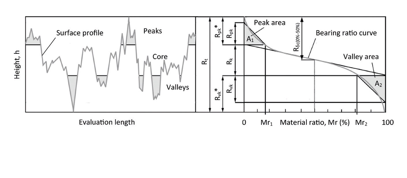 Figure 2. Surface profile and bearing ratio curve. Rt, total roughness height. Rk, core roughness height. Mr1 and Mr2, smallest and greatest material ratios, respectively, at the limits of the core roughness. Rpk*, highest peak height. Rpk, reduced peak height. A1, equivalent triangle peak area. Rvk*, deepest valley depth. Rvk, reduced valley depth. A2, equivalent triangle valley area. Rδc(0%-50%), height difference matching material ratios of 0 and 50%. Reproduced from Ref. 3 with kind permission.
The final step is to reformulate the Archard equation in terms of these new quantities. The original form is:
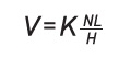
where
V is the worn volume,
N is the load,
L is the sliding distance,
H is the hardness and
K is the dimensionless wear coefficient. Normalizing by the contact area, replacing the sliding distance with a product of speed and time, absorbing the hardness into a new dimensional wear coefficient and expressing the equation in terms of decreasing height rather than increasing depth leads to:
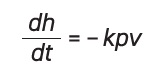
where
t is the time,
k the dimensional wear coefficient
(K/H), p the nominal contact pressure and
v the sliding speed. This is the equation for steady-state rubbing. However, during the running-in period, the only difference is that the contact area changes (according to the value of
Mr), and for a constant load, this leads to a change in pressure as
Mr changes from 0% to 100%. Taking this into account leads to:
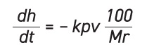
Substituting for
Mr yields:
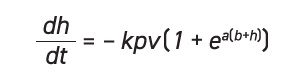
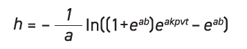
Solving with an initial condition of
h = 0 at
t = 0 yields an extended Archard equation that can define wear coefficients or predict wear if wear coefficients are known, regardless of the wear duration:
Varenberg went on to test his extended Archard equation by wearing polytetrafluoroethylene (PTFE) against mild steel in a ring-on-block configuration, where the PTFE had been pre-roughened with sandpaper and then profiled to yield
a and
b. The results
(see Figure 3), which use
k values derived from the steady-state portion of the curve, show an impressive agreement between the predictions from the equation and the experimental results.
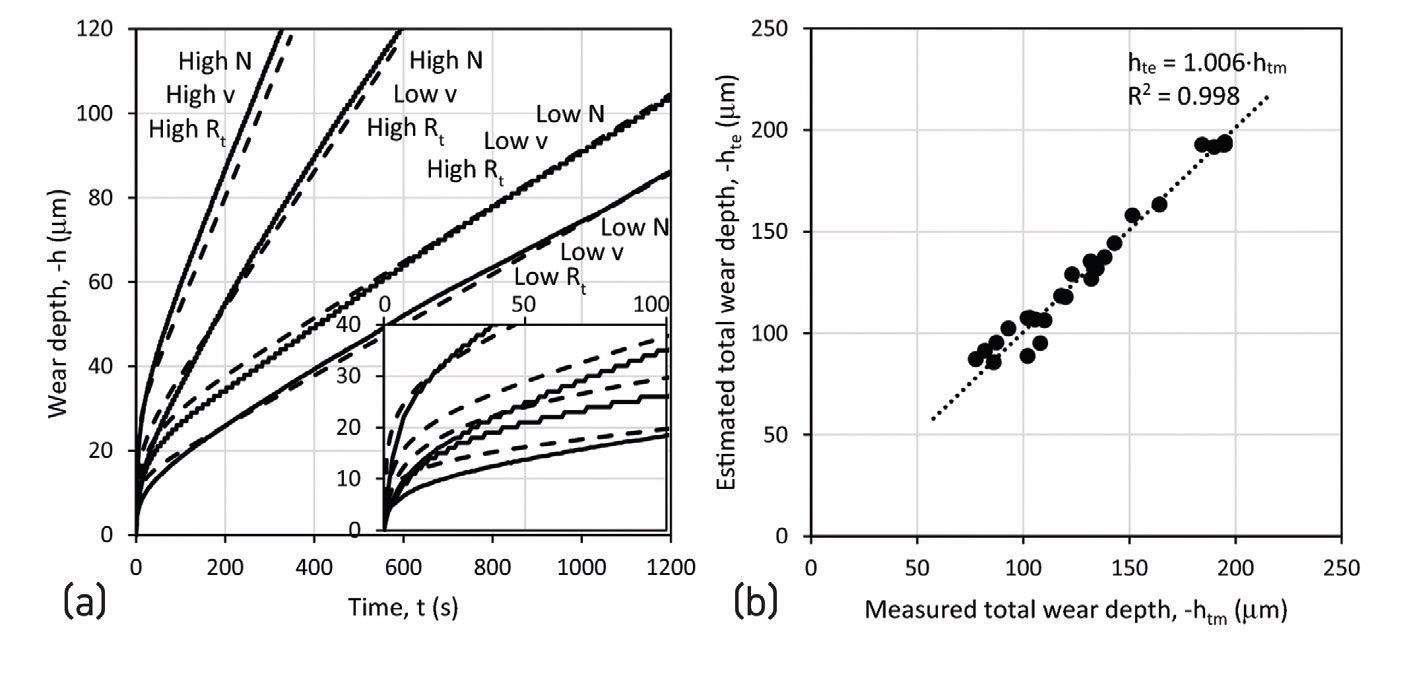 Figure 3. (a) Illustrative examples of the evolution of wear depth with time. Inset represents the close-up of the running-in period. Solid lines represent experimental data; dashed lines represent the model predictions. (b) Correlation of estimated and measured total wear depth in all experiments. Reproduced from Ref. 3 with kind permission.
This elegant piece of work convincingly shows that the already useful Archard equation can be extended into the running-in phase, thanks to the use of the bearing-ratio curve, the inclusion of a relatively simple piece of borrowed mathematics and the inclusion of profilometric measurements to obtain a couple of initial-surface roughness parameters.
REFERENCES
1.
Archard, J.F. (1953), “Contact and rubbing of flat surfaces,”
J. Appl. Phys., 24, pp. 981-988.
2.
Queener, C.A., Smith, T.C. and Mitchell, W.L. (1965), “Transient wear of machine parts,”
Wear, 8, pp. 391-400.
3.
Varenberg, M. (2022), “Adjusting for running‑in: Extension of the Archard wear equation,”
Tribology Letters, 70, 59.
4.
Abbott, E.J. and Firestone, F.A. (1933), “Specifying surface quality: a method based on accurate measurement and comparison,”
ASME Mech. Engr., 55, pp. 569-572.
5.
Bacaër, N. (2011), “Verhulst and the logistic equation (1838).” In: A Short History of Mathematical Population Dynamics, pp. 35-39. Springer, London.
Eddy Tysoe is a distinguished professor of physical chemistry at the University of Wisconsin-Milwaukee. You can reach him at wtt@uwm.edu.
Nic Spencer is emeritus professor of surface science and technology at the ETH Zurich, Switzerland, and editor-in-chief of the STLE-affiliated Tribology Letters journal. You can reach him at nspencer@ethz.ch.